Assessing Selected Teaching Techniques and Their Impact on Student Success in the Classroom
Timothy S. Faith, JD
From the Legal Studies Department, School of Business, Technology and Law, Community College of Baltimore County, Baltimore, Maryland.
Timothy S. Faith, JD
tfaith@ccbcmd.edu
ABSTRACT
Student success in college courses is important to students and faculty, though what variables predict student success are myriad and can be difficult to collect by faculty. Given the complex interaction of these variables, many of which are external to the classroom, a faculty member could be excused for thinking that the work of the faculty may not be impactful at all as to student success. However, this study considers several teaching techniques, including chunking course materials and assessments into smaller units, expanding practice homework assignments, and automating some course feedback to students through software, and identifies that increasing the number of exams that cover smaller portions of material appears to increase the average student pass rate of exams, but expanding homework and automating course/assignment feedback to students does not significantly impact student average exam grades. However, the use of intelligent agents did appear to negatively impact the rate at which students completed all exams in the course.
INTRODUCTION
Business Law I is a 3-credit survey course in the management program. As a survey course on business law, a variety of topics are included: constitutional law, the court system, torts, criminal law, contracts, uniform commercial code, intellectual property, business ethics, and agency and employment law. A variety of teaching techniques have been employed in the course. A natural question is whether any of these teaching techniques or assignments have a positive impact on student learning and success in the course.
To evaluate this question, the following observational study was developed that examines student learning outcomes in the form of average exam scores in relation to the implementation of several teaching techniques, including: chunking homework and assessment of materials in the course into smaller portions, the use of a journaling assignment to invite students to extend their knowledge through independent research on concepts introduced in the course, and the use of automation for student follow-up on attendance, missed assignments, and success. Additionally, the study examines whether the use of intelligent agents within the learning management system (LMS) impacts the rate at which students complete all exams in the course.
METHODS
Student learning in the Business Law course has generally been assessed based on course exams. Student success rates (defined as those students earning an ABC grade) vary in the study period with an average success rate of 53% in the course (including students that withdrew) as described in Table 1.
| Table 1. Summary of Success Rates (ABC) by Calendar Year. | |||||
|---|---|---|---|---|---|
| 2016 | 2017 | 2021 | 2022 | Total | |
| Success Rate | 62% | 65% | 44% | 48% | 53% |
| N | 125 | 131 | 164 | 174 | 594 |
The following were treatments implemented during the study period, and the success rates of each treatment are summarized in Table 2:
- Assessment using 4 exams rather than 3 exams during the semester in an effort to chunk materials into smaller portions;
- Expansion of homework problem sets (multiple choice questions related to course materials) from 6 sets to 12 so that student homework would also be chunked into smaller portions; and
- Implementation of intelligent agents within the LMS to message students automatically based on certain conditions.
| Table 2. Summary of Success Rates by Treatment. | |||
|---|---|---|---|
| Intervention | Success Rate | N | |
| Problem sets | 6 or fewer problem sets (control) | 55% | 465 |
| 12 problem sets (treatment) | 47% | 129 | |
| Assessments | 3 exam format (control) | 58% | 275 |
| 4 exam format (treatment) | 49% | 319 | |
| Intelligent agents | No intelligent agents (control) | 54% | 510 |
| Use of intelligent agents (treatment) | 51% | 84 | |
A summary of which sections of students were included in the control or treatment group for each of the above treatments is described in Table 3. Treatments (a) and (b) were originally inspired by a study by Humphries and Clark (2021), which suggested that students preferred shorter lectures and chunked course materials over longer lectures. Research by Fulkerson and Martin (1981) suggested that having shorter but more frequent quizzes may correlate with higher average scores, though such students did not do better on average on a cumulative final exam as compared to students with larger but less frequent quizzes during the semester. With regards to treatment (b), a wider educational debate exists as to the merits of homework generally and its impact on student achievement, as discussed by Trautwein (2007). Trautwein states that an increase in homework frequency was a significant predictor of achievement at the class level in study 2 of a multi-level model developed based on data collected for a larger international study. In study 2, data were collected from 2,216 German mathematics students in 91 classes, and a positive, significant relationship was found between homework effort by students and success on mathematics exams in study 3 discussed in the same paper. Similarly, Bowman et al. (2014) reported that higher average time spent on online chemistry homework correlated with improved exam and course grades.
| Table 3. Student Groupings into Control and Treatment Groups. | ||
|---|---|---|
| Control Sections | Treatment Sections | |
| 4 unit exams |
|
|
| 12 problem sets |
|
|
| Intelligent agents used |
|
|
With regards to treatment (c), the use of automated reminders was studied in a small sample of math and economics students, and the authors found an increase in completion rates compared to a control group not exposed to the reminder software (Carmean & Frankfort, 2013). A separate study with the same software at a community college found an increase in retention rates from fall to spring when comparing students exposed to the reminder system with students that served as the control group (Maslin et al., 2014). Other authors studied the use of email and text message reminders to students with a flipped classroom, and found that the “consistent nudging via text messages appears to be pivotal in ensuring student success” (Sherr et al., 2019). These authors concluded that text messaging was significantly related to student success and retention when such messages were sent consistently.
The present study is observational rather than a randomized controlled trial because students could not be randomly assigned to courses offered as this would be impractical for college enrollment (Adelson, 2013). Observational studies create a strong possibility of bias due to confounders in the observed data, where a baseline covariate within the population may be the true cause of the observed result, rather than the treatment being analyzed by the study (Austin, 2011). In a randomized controlled trial, an unbiased estimate of the average treatment effect can be calculated by a difference of the means of outcomes between the control and treated populations. However, an observational study’s control and treatment groups may vary such that other covariates, including, for example, the age, family income, or race distribution of each group, may bias the difference between the observed means. One methodology discussed in the literature to counter this problem is the use of a propensity score.
Rosenbaum and Rubin (1983) originally developed the propensity score as expressed in the following formula: ei = P r (Zi = 1|Xi), where ei is the preference score of the individual, i, Xi is a vector of features or characteristics for individual i, and Zi is a binary variable indicating whether or not individual i is a match. The purpose of calculating a propensity score is to create a similar treatment and control group so that the distribution of known covariates is similar between the groups, “[T]hus, in a set of subjects all of whom have the same propensity score, the distribution of observed baseline covariates will be the same between the treated and untreated subjects” (Austin, 2011). Fischer’s (2015) implementation of propensity score matching (PSM) was “to create subsets of students who were statistically similar across three important covariates: age, gender, and minority status” by regressing the bivariate treatment condition on these covariates and matching using “nearest neighbor matching with calipers” to create homogenous treatment and control groups.
Predictors of student success in college courses have been extensively studied in the literature. Alyahyan and Düştegör (2020) identified numerous factors from prior research that may correlate with student success, including past student performance such as high school grade point average (GPA) and/or student GPA in prior college courses; student demographics such as gender, race, and socioeconomic status; the type of class, semester duration, and program of study; psychological factors of the student such as student interest, stress, anxiety, and motivation; and e-learning data points such as student logins to the LMS and other student LMS activity.
An initial dataset of 594 enrollments was collected from students enrolled in my Business Law courses from sections taught in Spring 2016, Fall 2016, Spring 2017, Fall, 2017, Spring 2021, Fall 2021, Spring 2022, Summer 2022, and Fall 2022. Enrollments included students that completed the course, along with students that withdrew before completion. The 5 students that withdrew from the course are excluded from this analysis, as data for these students was unavailable. Data collected included average score on exams in the course, whether the class was taught in person/remote synchronously, whether the class was a full-term (14-week) course, whether the student was male, overall credit hours attempted by the student, and overall GPA of the student. GPAs were grouped into categories to simplify the matching process. GPA >3.75 was grouped as 4, GPA between 3.25 and 3.75 was grouped as 3.5, GPA between 2.75 and 3.25 was grouped as 3, GPA between 2.25 and 2.75 was grouped as 2.5, GPA between 1.75 and 2.25 was grouped as 2, GPA between 1.25 and 1.75 was grouped as 1.5, GPA between 0.75 and 1.25 was grouped as 1, GPA between 0.25 and 0.75 was grouped as 0.5, and below 0.25 the GPA was defined as 0.
The following dependent variables were defined: whether the student received a passing average exam grade (an average of at least 60%), the final grade in the course (A grades were coded as 4, B as 3, C as 2, D as 1, and other grades as 0), and whether the student completed all of the exams in the course. The following treatments were defined: isTreatmentPST1 (whether the student had a total of 12 problem sets during the course, or had 6 or fewer problem sets), isFourExamsT1 (whether the student had 4 exams with 1 for each of the 4 units, or whether the student had 3 exams where the unit exams on contracts were combined), and isTreatmentAAT1 (whether intelligent agents were used in the course).
A subset of data was defined for students who had at least 12 attempted credit hours and attempted all of the exams in the course of 395 student enrollments. The purpose of this subset was to identify the student’s prior performance at the college by the student’s cumulative GPA, which prior research identifies as an important covariate related to student success (Alyahyan & Düştegör, 2020).
A linear regression model was defined, looking for a relationship between average exam grades and the treatments above, along with several independent variables. The result of each of these models is described in Tables 4, 5, and 6, below. Several covariates discussed below seem to confound whether the treatments studied in these models were the cause of the variation in student performance or completion. To control for confounding covariates, PSM was implemented for this subset of students using the MatchIt library within R. PSM was used to estimate the Average Treatment Effect on the Treated (ATT) for 3 treatments noted above on average student exam scores by using the comparisons function within the MarginalEffects library. This function takes as input each preference score-matched model, and compares that with a subset of the treated observations to provide an estimated ATT. A total of 3 models were defined (4 Exams, 12 Problem Sets, and Intelligent Agents) to evaluate the ATT.
| Table 4. Effects of Select Variables on Exam Scores. | ||
|---|---|---|
| Estimated effect on average exam score | p value | |
| 4 exams | +0.05 | 0.02* |
| 12 problem sets | -0.02 | 0.26 |
| Online students | -0.03 | 0.02* |
| Full term students | -0.05 | 0.02* |
| Remote synchronous students | -0.04 | 0.08 |
| Male students | +0.03 | 0.0003*** |
| Intelligent agents used | -0.05 | 0.004** |
| Overall GPA | +0.09 | >0.001*** |
| Overall hours attempted | 0 | 00.46 |
| Significance: * 0.05, ** 0.001, *** 0.0001.
F = 19.16, adjusted R-squared = 0.3154. |
||
| Table 5. Effects of Select Variables on Pass Rates. | ||
|---|---|---|
| Estimated effect on overall pass rate | p value | |
| 4 exams | +0.04 | 0.640 |
| 12 problem sets | -0.003 | 00.961 |
| Online students | -0.07 | 0.446 |
| Full term students | -0.09 | 0.261 |
| Remote synchronous students | +0.07 | 0.445 |
| Male students | +0.07 | 0.057 |
| Intelligent agents used | +0.05 | 0.489 |
| Overall GPA | +0.32 | >000.1*** |
| Overall hours attempted | 0 | 0.667 |
| Significance: *** 0.0001.
F = 14, adjusted R-squared = 0.2433. |
||
| Table 6. Effects of Select Variables on Grades. | ||
|---|---|---|
| Estimated effect on letter grade | p value | |
| 4 exams | +0.21 | 0.200 |
| 12 problem sets | +0.10 | 0.517 |
| Online students | -0.25 | 0.026* |
| Full term students | -0.08 | 0.576 |
| Remote synchronous students | +0.12 | 0.502 |
| Male students | +0.16 | 0.028* |
| Intelligent agents used | -0.11 | 0.376 |
| Overall GPA | 1.10 | >0.0001*** |
| Overall hours attempted | 0 | 0.414 |
| Significance: * 0.05, *** 0.0001.
F = 42, adjusted R-squared = 0.510. |
||
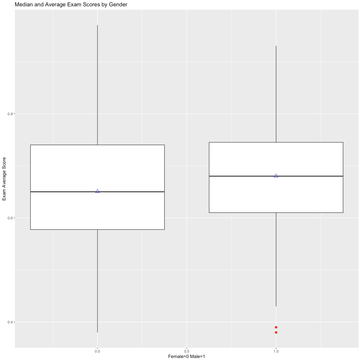
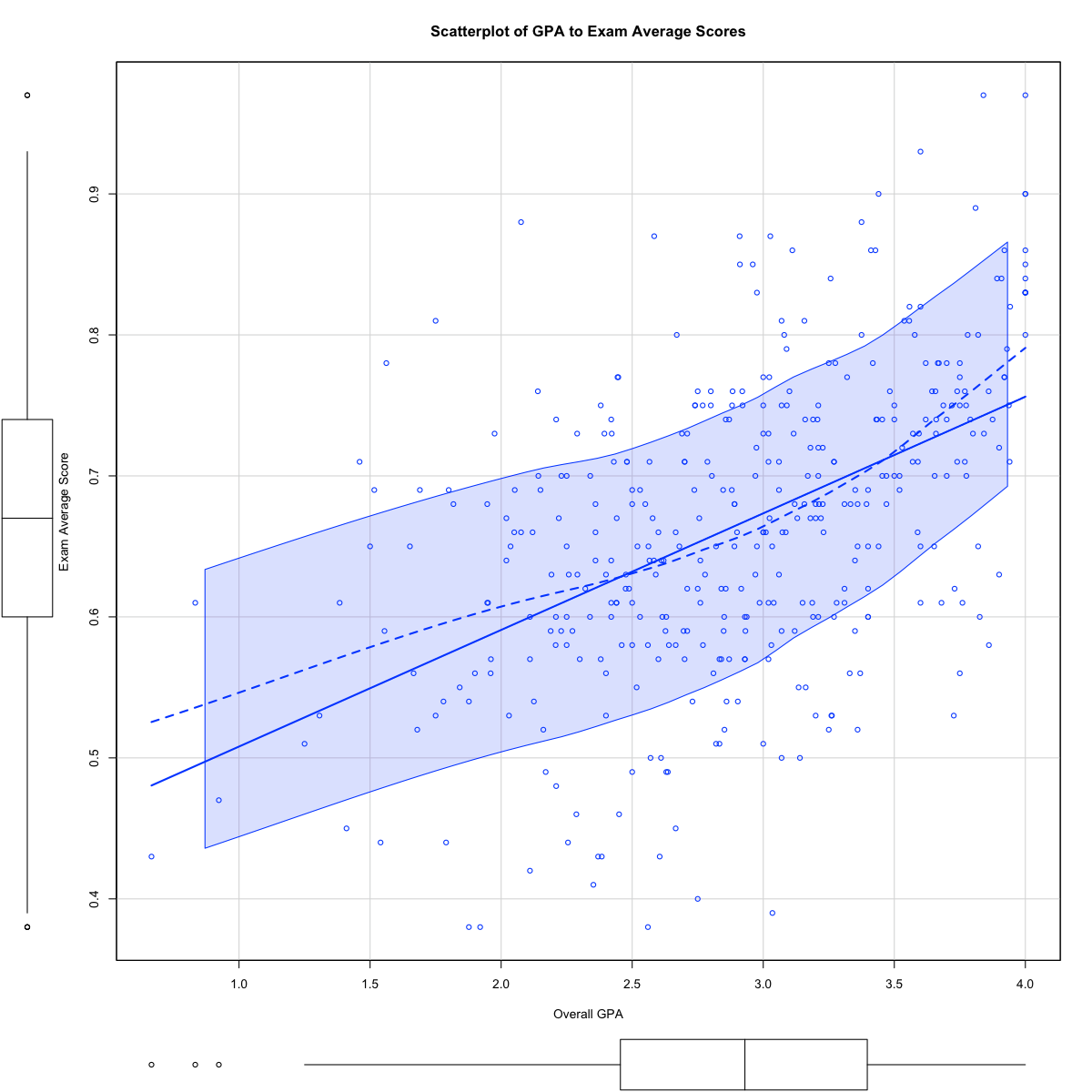
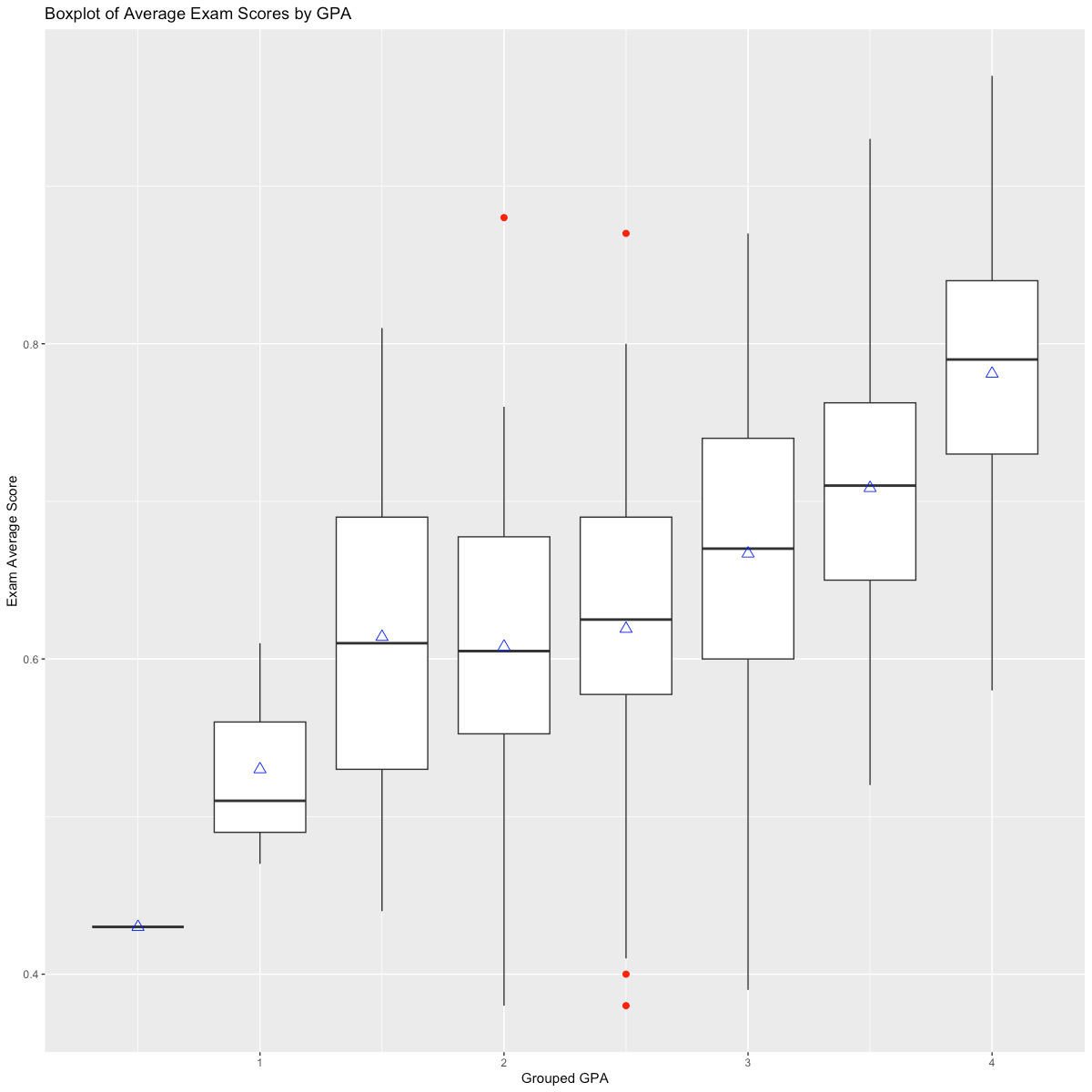
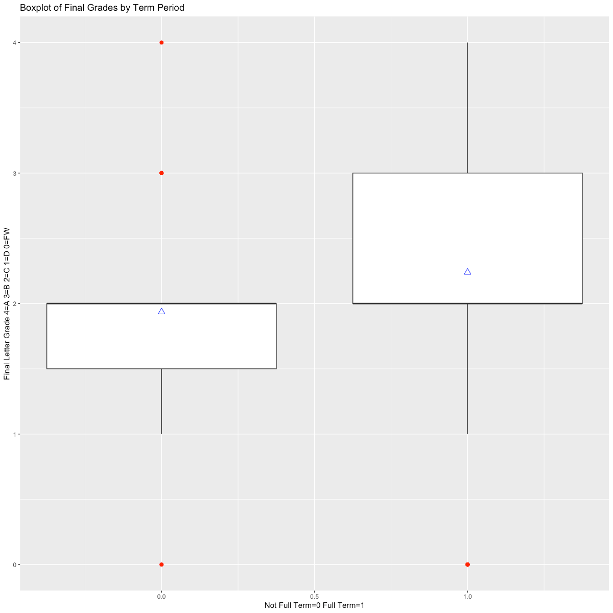
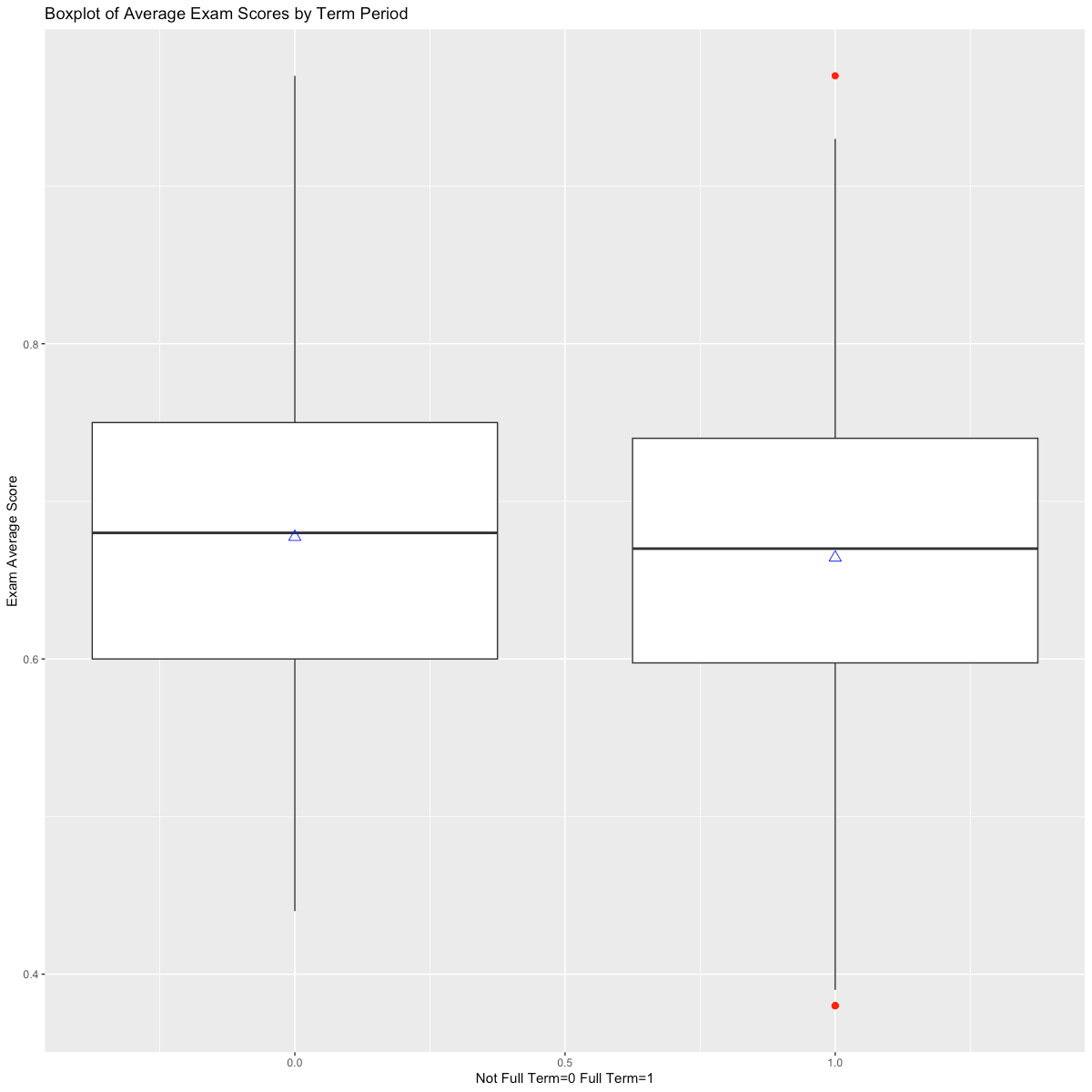
In defining the PSM models, I investigated variations in student outcomes based on available independent variables, noting that male students tended to have a higher average exam score than female students (Figure 1A), and that a correlation of higher exam scores and higher cumulative grouped GPA was present in the data (Figures 2 & 3A). These correlations persisted when examining the overall final grade in the course. In addition, I noted that full-term students, which are those students that completed the course in a traditional 14-week period, had a higher mean and median final grade in the course compared to students that took the course in a compressed period (Figure 3B), though this was reversed when examining average exam grades (Figure 3C).
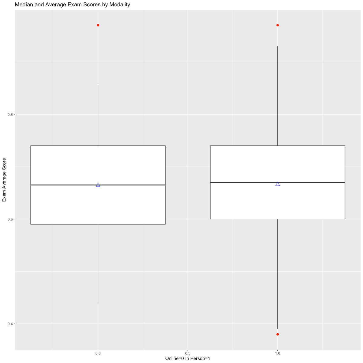
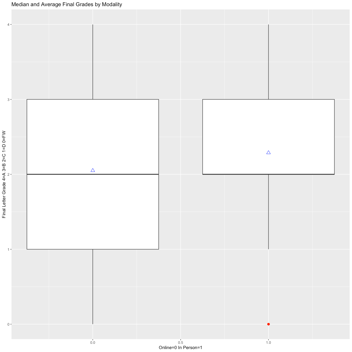
I also investigated whether average exam scores might be related to whether the course was taught in person, and found that there was a small variation on the mean or median for this independent variable (Figure 1B), however a substantial difference was found for overall student grades based on modality (Figure 1C). Independent variables that showed variation on the mean of a dependent variable were used in matching for each of the PSM models on the premise that balancing students between control and treatment groups would improve the overall reliability of the models for further analysis.
All of the models described below used whether the class was in person, the grouped GPA of the student, whether the student was male, and whether the class was a regular, 14-week term to match treatment with control enrollments. I first attempted 1:1 nearest neighbor PSM without replacement with a propensity score estimated using logistic regression of the treatment on the covariates and also genetic PSM with a population size of 1,000 (Griefer, 2022), but both of these methods resulted in poor balance. Instead, I implemented a “full” PSM, which had an adequate balancing for the 4 Exams, 12 Problem Sets, and Intelligent Agent models, as more fully described in Figures 6, and 7A and 7B for these models (Austin, 2010; Ho, 2011).
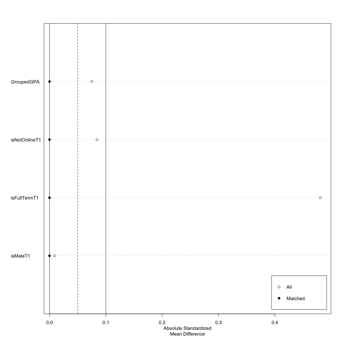
One additional model was defined to examine whether the use of intelligent agents had an impact on students taking all the exams in the course for students who had attempted at least 12 credit hours at the college using 537 enrollments. Figure 7C illustrates the resulting balance obtained using exact matching for this model. The matching for the Intelligent Agent model resulted in discarding 86 control and 3 treatment observations from the model.
After matching, all standardized mean differences for the covariates were below 0.1 and all standardized mean differences for squares and 2-way interactions were below 0.15. Full matching meant that all treated enrollments were matched with a control enrollment, so no enrollments were discarded by the matching procedure for the first 3 models. Exact matching resulted in discarding 3 control units, though this loss was acceptable as the overall balance of the model was achieved (Austin, 2011).
To estimate the treatment effect and its standard error for each model, I fit a linear regression model with whether the student passed the exams (an average score on the exams of at least 60%) as the outcome, and the treatment, covariates, and their interactions as predictors, and then included the full matching weights in the estimation. The “lm” function was used to fit the outcome, and the comparisons function in the marginaleffects library was used to perform a g-computation in the matched sample to estimate the ATT (Griefer, 2022).
The source data for the study was collected from instructor grade books for each of the semesters noted above and was imported into a MySQL database. Data on students that withdrew was collected separately from institutional data sources. Certain variables, such as student gender, overall credit hours attempted, and cumulative GPA were collected from institutional data sources. The open source statistical package, R version 4.2.2, was used for multivariable linear regressions, preference score matching analysis, and Love, Scatterplots, and density plots were created using the libraries RMySQL, MatchIt, Cobalt, ggplot2, and MarginalEffects.
RESULTS
Table 2 summarizes student success rates in the course for certain variables, without any regression or PSM applied to the dataset. The reader will note that at first blush, the treatments applied within the course do not appear to yield a higher success rate when compared to a control group to which the treatment was not applied. However, this result could simply be by chance. Therefore, an initial multivariable model was developed, to which a linear regression was applied in an effort to determine which independent variables, including both fixed effects (such as the student’s gender, class modality, class term) and random effects (such as the treatments applied, student overall credit hours attempted and student cumulative GPA). Table 4 summarizes this initial regression. This regression suggests that some of these variables are significantly related to average student exam results, including having 4 exams rather than 3 (p = 0.02), and using intelligent agents (p = 0.005), while other treatments like more homework problem sets are not significantly related. The regression also strongly suggests that there is a significant relationship between cumulative GPA of students and average student exam results. The scatterplot in Figure 1A illustrates that higher GPAs tend to cluster with higher average exam scores, consistent with Tables 4, 5, and 6.
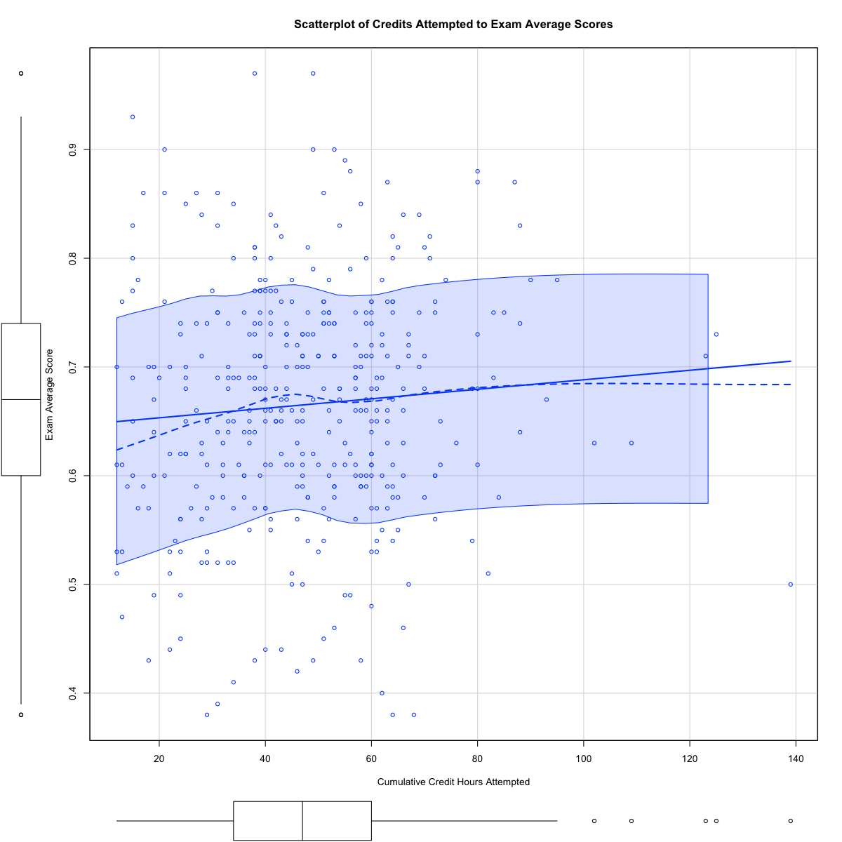
In contrast, no pattern emerges in the scatterplot in Figures 1A and B when plotting cumulative credits attempted by the student and average student exam scores, also consistent with the analysis presented in Tables 4, 5, and 6. The inference of this data is that just exposure to college courses does not correlate with performance in college courses, though prior success in college courses may correlate with future student success.
A regression was also constructed to compare the overall success rate (students earning an ABC) in the course with same variables as above, the results of which are reported in Table 5. Of note is the fact that no variables are significantly related to the overall course pass rate, except the student’s cumulative GPA (p > 0.0001). Drilling a bit deeper, a final regression was constructed to examine individual letter grades received in the course with the same variables, the results of which are reported in Table 6, where the final letter grade was assigned a number from 0 to 4, with A=4, B=3, C=2, D=1, and all other grades, 0. This analysis suggests that online students had a significantly lower letter grade compared to non-online students (p = 0.03), though the analysis also suggested that cumulative GPA is significantly correlated with a higher letter grade in the course (p > 0.001).
However, as noted above, observational studies may be biased by baseline characteristics of persons included in the study, such that certain characteristics in the population better predict the dependent variable than the treatments studied. As noted above in the literature and the above regression models, prior GPA is a strong predictor of student success in subsequent courses and likely is an important covariate that would improve the clarity of the analysis if properly controlled for through an alternate statistical method (Austin, 2011). Austin notes several other educational researchers that have used PSM to address this concern. Fischer (2015) also uses PSM in a study of the use of open educational resources in an observational study of the impact of such resources on student performance to better control for the uneven distribution of certain student characteristics that tend to predict student success.
A question arises as to whether there is an uneven distribution of students based on cumulative GPAs among the control and treatment groups included in this data subset. There appears to be a declining trend in the average GPA of students taking the course as described in Figure 5. This trend may be an important confounding covariate that may better explain student performance rather than the treatments implemented in the course, given that many of the control enrollments are sourced from when student average cumulative GPA was higher. To try to balance control and treatment groups with similar students, I implemented PSM using the R “matchit” function, for the purpose of calculating an estimated ATT for each of the 4 treatments in the study.
The 4-Exams Model was used to evaluate the ATT associated with using 4 exams to assess student learning, rather than 3. Figure 6 is a density plot illustrating the balance of the model after matching compared with the unbalanced starting data. The estimated effect was 0.162 (SE = 0.0413, p > 0.001), indicating that students who completed 4 unit exams on average were more likely to earn a passing average exam grade compared to students who were assessed using 3 unit exams.
The 12 Problem Sets model was used to evaluate the ATT associated with the use of additional homework and its impact on the average student exam pass rates. Figure 7A is a Love plot illustrating the balance of the model after exact matching between the treatment and control observations. The estimated effect was -0.0036 (SE = 0.0616, p = 0.95), indicating that having more problem sets as homework assignments probably had no impact on the frequency at which students passed the exams on average in the course.
The Intelligent Agents model was used to evaluate the ATT associated with sending automated reminders to students concerning attending to the course, advising students when they missed an assignment, and encouraging students to reach out when they did poorly on one or more assignments during the semester, and the impact of this messaging on average student exam pass rates. Figure 7B is a Love plot illustrating the balance of the model after using subclass matching between treatment and control observations. The estimated effect was 0.0303 (SE = 0.0587, p = 0.61), indicating that the use of automated agents did not have any significant impact on the average student pass rate of the exams.
The careful reader will note that the initial pool of students (n = 594) is substantially larger than those included in the above analysis (n = 395) of the 3 treatments on average exam pass rates for those that took all the exams. A substantial subset of students (51) withdrew from the course as summarized below in Table 7 and a substantial subset of students (177) did not complete all exams in the course. For students (56) with less than 12 attempted credit hours, less than half (21/56) completed all exams, and the majority (38) failed or withdrew from the course.
| Table 7. Withdrawal Rates by Semester. | ||||||||||
|---|---|---|---|---|---|---|---|---|---|---|
| Spring 2016 | Fall 2016 | Spring 2017 | Fall 2017 | Spring 2021 | Fall 2021 | Spring 2022 | Summer 2022 | Fall 2022 | Total | |
| Withdrawals | 3 | 4 | 5 | 3 | 4 | 12 | 7 | 0 | 13 | 51 |
| Did not take all exams | 7 | 6 | 15 | 4 | 22 | 26 | 23 | 6 | 18 | 127 |
| Took all exams | 44 | 61 | 61 | 44 | 78 | 32 | 43 | 15 | 49 | 417 |
| Withdrawal rate | 5.6% | 5.6% | 6.2% | 5.9% | 3.8% | 17.1% | 9.6% | 0% | 16.3% | 8.9% |
These raw numbers indicate a substantial student loss rate across the study period of approximately 47% (students that earned a DFW as a percent of all students enrolled), with a notable increase in the withdrawal rate starting in 2021 compared with the 2016 and 2017 semesters included in the study as indicated in Table 7. Superficially, one might conclude that the treatments implemented in 2021-2022 may be exacerbating withdraw and/or failure rates in the course.
I therefore studied whether a treatment that increased teacher-student interactions might increase the rate at which students completed all exams in the course (Cifuentes & Lents, 2010). Several other researchers studied the use of automated reminders and found that these resulted in improved student outcomes and retention (Carmean & Frankfort, 2013; Maslin et al., 2014; Sherr et al., 2019). The Intelligent Agents model involves messaging students who are not logging into the course weekly, and also sending students automated feedback on certain homework assignments during the semester, resulting in increased teacher-student interactions through course messaging beyond course announcements and automated calendar reminders within the LMS. I studied the effect of intelligent agents on students completing all exams in the course. After matching, the Love plot in Figure 7C illustrates balancing of the matched model. The estimated effect was -0.12 (SE = 0.0448, p = 0.008), indicating that the use of automated agents significantly reduced by 12% the frequency at which students completed all the exams.
DISCUSSION AND CONCLUSION
Breaking up assessments in the course into 4 units from 3 seems to increase exam pass rates by approximately 16%, while the other 2 treatments did not seem to have a significant effect on the average exam pass rate of students who took all the exams during the course and attempted at least 12 credit hours at the college. However, the use of intelligent agents appears to have significantly reduced the rate at which students completed all the exams in the course by 12%, suggesting that the additional reminders may have been discouraging. This may be the result of messaging-overload for students that were struggling to keep up with the class, discouraging them from attempting all of the exams.
As noted above, there are myriad variables that may have some statistical significance to student success, though not all of these variables could reasonably be included in the present study. A follow-up study on these preliminary findings may expand the control and treatment groups to include additional observations to improve the overall matching using larger pools, and also to include additional independent variables from institutional research sources for these students which may contribute to student performance. For example, collecting data on student performance in 2014-2015 and 2018-2020 may help to expand both control and treatment groups to improve matching performance and reliability. Also, collecting data on race/ethnicity, student age, student poverty status, student motivation, and student LMS usage may better explain variations in student outcomes and may result in better matches between control and treatment groups, and a better estimate of the ATT of any particular treatment considered in the study.
The bulk of this study is focused on students with sufficient credit hours at the college to establish a base cumulative GPA; the remaining sample of students was not studied as student GPA prior to work at the college was not available for this study. Such students that are new to college courses may be an important population to study in a separate analysis with additional data, including student high school GPA and other variables that are strongly correlated with student performance. Conclusions reached here may not be more generalizable outside of the context of a business law course when the course subject matter does not lend itself to a combination of lecture and student discussion of scenarios applying law concepts. Finally, some of the students in the treatment groups were exposed to more than one treatment concurrently and the combinations of treatments may impact average student exam scores and/or the rate at which students complete all exams in the course, however, this was not studied.
REFERENCES
- Alyahyan, E., & Düştegör, D. (2020). Predicting academic success in higher education: literature review and best practices. International Journal of Educational Technology in Higher Education, 17, Article 3. https://doi.org/10.1186/s41239-020-0177-7
- Austin, P. C. (2011). An introduction to propensity score methods for reducing the effects of confounding in observational studies. Multivariate Behavioral Research, 46(3), 399-424. https://doi.org/10.1080/00273171.2011.568786.
- Bean, J. C. (2001). Engaging ideas: The professor’s guide to integrating writing, critical thinking, and active learning in the classroom (1st ed.). Jossey-Bass/Wiley.
- Bowman, C. R., Gulacar, O., & King, D. B. (2014). Predicting student success via online homework usage. Journal of Learning Design, 7(2), 47-61. http://dx.doi.org/10.5204/jld.v7i2.201
- Barkley, E. F. (2010). Student engagement techniques: A handbook for college faculty. Wiley.
- Carmean, C., & Frankfort, J. (2013). Mobility, connection, support: Nudging learners to better results. EDUCAUSE Review. http://www.educause.edu/ero/article/mobility-connection-support-nudging-learners-better-results
- Cifuentes, O. E., & Lents, N. H. (2010). Increasing student-teacher interactions at an urban commuter campus through instant messaging and online office hours. Electronic Journal of Science Education, 14(1), 1-13.
- Fulkerson, F. E., & Martin, G. (1981). Effects of exam frequency on student performance, evaluation of instructor, and test anxiety. Teaching of Psychology, 8(2), 90-93. https://doi.org/10.1207/s15328023top0802_7
- Goacher, R. E., Kline, C. M., Targus, A., & Vermette, P. J. (2017). Using a practical instructional development process to show that integrating lab and active learning benefits undergraduate analytical chemistry. Journal of College Science Teaching, 46(3), 65-73.
- Griefer, N. (2023, June 13). MatchIt: Getting started. https://cran.r-project.org/web/packages/MatchIt/vignettes/MatchIt.html#assessing-the-quality-of-matches
- Ho, Daniel, Imai, Kosuke, King, Gary, Stuart, Elizabeth A. (2011) MatchIt: Nonparametric Preprocessing for Parametric Causal Inference. https://r.iq.harvard.edu/docs/matchit/2.4-20/matchit.pdf
- Humphries, B., & Clark, D. (2021). An examination of student preference for traditional didactic or chunking teaching strategies in an online learning environment. Research in Learning Technology, 29. https://doi.org/10.25304/rlt.v29.2405
- Maslin, A., Frankfort, J., Jaques-Leslie, M. (2014). Mobile supports for community college students: Fostering persistence through behavioral nudges. League for Innovation in the Community College.
- Roback, P., Legler, J. (2021). Beyond multiple linear regression: Applied generalized linear models and multilevel models in R. Chapman & Hall. https://bookdown.org/roback/bookdown-BeyondMLR/
- Rosenbaum, P. R., & Rubin, D. B. (1983). The central role of the propensity score in observational studies for causal effects. Biometrika, 70(1), 41-55. https://doi.org/10.1093/biomet/70.1.41
- Sherr, G. L., Akkaraju, S., Atamturktur, S. (2019). Nudging students to succeed in a flipped format gateway biology course. Journal of Effective Teaching in Higher Education, 2(2), 57-69. https://doi.org/10.36021/jethe.v2i2.51
- Trautwein, U. (2007). The homework-achievement relation reconsidered: Differentiating homework time, homework frequency, and homework effort. Learning and Instruction, 17(3), 372-388. https://doi.org/10.1016/j.learninstruc.2007.02.009.
- Winitzky-Stephens, J. R., & Pickavance, J. (2017). Open educational resources and student course outcomes: a multilevel analysis. International Review of Research in Open and Distributed Learning, 18(4), 1-15. https://doi.org/10.19173/irrodl.v18i4.3118
- Zhao, Q., Luo, J., Su, Y., Zhang, Y., Tu, G., & Luo, Z. (2021). Propensity score matching with R: conventional methods and new features. Annals of Translational Medicine, 9(9), 812. https://atm.amegroups.com/article/view/61857